Chapter 4 Data i/o
4.1 Konzeptuelles
R kann mit vielen verschiedenen Datenobjekten zugleich umgehen. Es gibt Befehle für den Umgang mit einzelnen (Daten-)Objekten und Befehle für Bündel von (Daten-)Objekten in R. Alle zu einem Zeitpunkt bekannten (Daten-)Objekte sind im “Global Environment” zu finden (RStudio oben rechts “Environment”).
Alle zu einem Zeitpunkt in einer R-Session bekannten Daten (environment) können als Gesamtheit gespeichert und geladen werden (.RData). Dies betrifft nicht nur Datentabellen oder besser Datenobjekte, sondern auch alle anderen Objekte, beispielsweise Ergebnisobjekte (Analyseergebnisse). R-Projekte haben jeweils ein eigenes Environment, RData-Dateien sind also ein geeigneter Weg, verschiedene Umgebungen, z. B. verschiedene Analysen, voneinander getrennt in unterschiedlichen Projekten zu handhaben.
Einzelne Datenobjekte (Tabellen, Vektoren) können dem “Global Environment” hinzugefügt werden über Befehle oder auch interaktiv in RStudio. Viele Formate können eingelesen werden, gängig sind z. B. Spreadsheets (MS Excel, Libreoffice Calc), also *.CSV oder *.xlsx. Datentabellen anderer Statistikprogramme wie SPSS, SAS usw. können ebenfalls eingelesen werden, ggf. mit Hilfe spezieller Packages wie library(foreign) oder das library(readr) aus dem tidyverse. Auch Datenbankabfragen, z. B. SQL, sind als Datenquelle möglich.
Datenobjekte bzw allgemein R-Objekte können neben den eigentlichen Daten auch Metainformationen enthalten. Sie sind gespeichtert in den Properties der jeweiligen Objekte. Die Properties kann man in RStudios “Global Environment” aufklappen und inspizieren.
Das Schreiben einzelner Datenobjekte, z. B. einer einzelnen Datentabelle aus dem “Global Environment” wird in RStudio nicht interaktiv unterstützt. Dies ist aber über R-Kommandos möglich.
Daten können auch von einem R-Skript automatisiert über eine URL aus dem Internet gelesen werden.
Wir stellen eine Möglichkeit vor, einzelne Datenobjekte wie eine einzelne Datentabelle mit all ihren R-Eigenschaften (Properties) einzulesen, auch über URL, bzw. wegzuschreiben.
4.2 R Environment - .RData
- finden
- lesen
- schreiben
- der Bezug zum “working directory”
- in Projekten
Die Extension *.RData kennzeichnet Dateien, in der R-Environments gespeichert werden können bzw. aus denen ein R-Environment gelesen werden kann.
In einer RData-Dateien können viele verschiedene R-Objekte als Einheit verwaltet werden.
Default Name, z. B. bei save.image() ist .RData.
Hinweis: Unter Unix und auch unter MacOS sind Dateinamen, die mit einem Punkt beginnen, “hidden”, d. h. oft unsichtbar.
R-Projekte haben ein projektbezogenes Environment (siehe dort).
# it's always a good idea for file i/o to know our current working directory is
# this is, where files are looked for and saved at
getwd()
## [1] "/Users/pzezula/ownCloud/lehre_ss_2022/unit/b_data_mangling"# the whole current environment can be saved via
save.image() # this saves all objects in a file called .RData in the working directory
# we might also use a specific name
save.image(file="my_current_environment.RData") # this saves all objects in a file called my_current_environment.RData in the working directory
# restoring this environment can be done via
load("my_current_environment.RData")
# we can also save a selection of objects in a RData-file
# suppose, we have two data objects called heights and dd in our current environment
heights <- c(180, 170, 190)
dd <- data.frame(
subje = c(1,2,3),
heights = heights
)
# so we could save these two objects in a file called "1.RData" in the current working directory
save(heights, dd, file="1.RData")
# we could now delete the two objects from our environment
rm(heights, dd)
# if we want to load these two data objects in our current environment, we could use:
load(file="1.RData")4.3 Umgang mit einzelnen Datenobjekten
Auch wenn R mit multiplen Datenobjekten zugleich umgehen kann, liegen Daten häufig in zweidimensionaler Form vor mit Variablen als Spalten und Beobachtungen als Zeilen. Solche Datenstrukturen stammen oft aus Spreadsheets (Tablellenkalkulationen) wie MS Excel, auch weil dies komfortable Werkzeuge zur Dateneingabe sind und allererste Modifikationen und Visualisierungen erlauben.
4.3.1 Möglichkeiten interaktiv in RStudio
RStudio unterstützt den Import einzelner Datentabellen in die Arbeitsumgebung (environment) interaktiv.
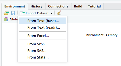
import_dataset
Das ist möglich und anfangs komfortabel. Die Idee reproduzierbarer Analysen aber fordert eine automatisierbare Möglichkeit über R-Befehle
RStudio bietet keine interaktive Möglichkeit, einzelne (Daten-)Objekte aus dem Environment zu speichern.
4.3.2 Einlesen und abspeichern einzelner Datentabellen
R ermöglicht vor allem auch über verschiedene Packages den Umgang mit vielen gängigen Datenformaten. Ein sehr üblicher Weg sind Dateien aus Tabellenkalkulationen wie MS-Excel mit verschiedenen Dateiformaten “.xlsx”, ”.csv”. Üblich sind auch andere, häufig Textformate, vor allem aus Geräten wie Eye-Trackern etc. Eine andere gängige Datenquelle sind Datenbanken (SQL etc.).
Die Dateien mit den Daten müssen gefunden werden. Sie werden über die Dateinamen angesprochen. Ohne weitere Pfadangabe werden Dateien im aktuellen Arbeitsverzeichnis gesucht (working directory). Mit expliziter Pfadangabe sind auch andere Speicherorte erreichbar. Wir empfehlen das Einlesen von Daten über URLs, die eigentlichen Dateien werden also über das Internet geholt.
Beispiele:
Einlesemöglichkeiten einer Datentabelle, die in verschiedenen Formaten vorliegt.
4.3.3 Standard R
Daten im Textformat können mit Befehlen der library(utils) des Standard R gelesen und geschrieben werden.
Das funktioniert lokal aber auch mit URLs als Datenquelle.
# our working directory - here is where everything is looked for and stored at ...
getwd()
## [1] "/Users/pzezula/ownCloud/lehre_ss_2022/unit/b_data_mangling"# reading a tab delimited text file from an URL
dd1 <- utils::read.delim("http://md.psych.bio.uni-goettingen.de/mv/data/div/stud.txt")
# we might want to store dd1 under locally in the working directory and name it "stud_local.txt"
utils::write.table(dd1, file="stud_local.txt", sep="\t", row.names=F)
# then we can read it again locally
dd2 <- utils::read.delim("stud_local.txt")
# head(dd1 == dd2)The common *.csv file format used by MS Excel is also possible
CSV-Dateien sind unterschiedlich, je nach Landeseinstellungen. Sie unterstützen entweder Komma oder Punkt als Trennzeichen für “Nachkommastellen”. “1.5” z. B. im englischsprachigen Umfeld vs “1,5” z. B. im Deutschen. Auch der Spaltenseparator ist unterschiedlich: “,” vs “;” Daher gibt es zwei Befehle.
# we read the same data in two CSV-Versions with two different commands
dd1 <- utils::read.csv("http://md.psych.bio.uni-goettingen.de/mv/data/div/stud_csv.csv")
# dd1.wrong <- read.csv("http://md.psych.bio.uni-goettingen.de/mv/data/div/stud_csv2.csv")
dd2 <- utils::read.csv2("http://md.psych.bio.uni-goettingen.de/mv/data/div/stud_csv2.csv")
# head(dd1 == dd2)
4.3.4 Tidyverse
Tidyverse hat das Sub-Package library(readr) cheat-sheet.
Auch hiermit sind die obigen Dateien lesbar.
Im library(readr) sind die Befehle mit “_” aufgebaut: utils::read.csv() entspricht readr::read_csv()
# our working directory - here is where everything is looked for and stored at ...
getwd()
## [1] "/Users/pzezula/ownCloud/lehre_ss_2022/unit/b_data_mangling"# reading a tab delimited text file from an URL
dd1 <- readr::read_tsv("http://md.psych.bio.uni-goettingen.de/mv/data/div/stud.txt")## Rows: 100 Columns: 13
## ── Column specification ─────────────────────────────────────────────────────────────────────────────────────────────
## Delimiter: "\t"
## chr (1): string
## dbl (12): no, height, shoe_size, weight, gender, birth_month, birth_year, statistics_grade, abitur, math_intense,...
##
## ℹ Use `spec()` to retrieve the full column specification for this data.
## ℹ Specify the column types or set `show_col_types = FALSE` to quiet this message.# we might want to store dd1 under locally in the working directory and name it "stud_local.txt"
readr::write_tsv(dd1, file="stud_local.txt")
# then we can read it again locally
dd2 <- readr::read_tsv("stud_local.txt")## Rows: 100 Columns: 13
## ── Column specification ─────────────────────────────────────────────────────────────────────────────────────────────
## Delimiter: "\t"
## chr (1): string
## dbl (12): no, height, shoe_size, weight, gender, birth_month, birth_year, statistics_grade, abitur, math_intense,...
##
## ℹ Use `spec()` to retrieve the full column specification for this data.
## ℹ Specify the column types or set `show_col_types = FALSE` to quiet this message.# head(dd1 == dd2)
# library(readr) also covers the csv format
# we read the same data in two CSV-Versions with two different commands
dd1 <- readr::read_csv("http://md.psych.bio.uni-goettingen.de/mv/data/div/stud_csv.csv")## Rows: 100 Columns: 13
## ── Column specification ─────────────────────────────────────────────────────────────────────────────────────────────
## Delimiter: ","
## chr (1): string
## dbl (12): no, height, shoe_size, weight, gender, birth_month, birth_year, statistics_grade, abitur, math_intense,...
##
## ℹ Use `spec()` to retrieve the full column specification for this data.
## ℹ Specify the column types or set `show_col_types = FALSE` to quiet this message.dd2 <- readr::read_csv2("http://md.psych.bio.uni-goettingen.de/mv/data/div/stud_csv2.csv")## ℹ Using "','" as decimal and "'.'" as grouping mark. Use `read_delim()` for more control.
## Rows: 100 Columns: 13── Column specification ─────────────────────────────────────────────────────────────────────────────────────────────
## Delimiter: ";"
## chr (1): string
## dbl (12): no, height, shoe_size, weight, gender, birth_month, birth_year, statistics_grade, abitur, math_intense,...
## ℹ Use `spec()` to retrieve the full column specification for this data.
## ℹ Specify the column types or set `show_col_types = FALSE` to quiet this message.# head(dd1 == dd2)Tidyvers hat auch ein Sub-Package library(readxl) mit dem auch das binäre Format von MS Excel Dateien gelesen werden kann,
also Dateien im Format *.xls oder *.xlsx.
Leider kann es nur lokale Dateien lesen, keine URLs.
Hierzu dient alternativ die library(openxlsx) mit dem Befehl openxlsx::read.xlsx()
# library(readxl) and library(readxlsx) cover the binary MS Excel format
dd1 <- openxlsx::read.xlsx("http://md.psych.bio.uni-goettingen.de/mv/data/div/stud.xlsx")
# we can store it locally in format xlsx
openxlsx::write.xlsx(dd1, "stud.xlsx")
# local xlsx files can read with package readxl
dd2 <- readxl::read_excel("stud.xlsx")
# head(dd1 == dd2)
4.3.5 Base R: Andere Dateiformate: SPSS
Als Beispiel für andere Dateiformate soll hier SPSS als Quelle dienen:
Mit library(foreign) des Base-R können wir auch andere Formate einlesen, z. B. SPSS *.sav Dateien
dd <- foreign::read.spss("http://md.psych.bio.uni-goettingen.de/mv/data/div/stud.sav", to.data.frame=T)
head(dd)
## no height shoe_size weight gender birth_month birth_year statistics_grade abitur math_intense academic_background
## 1 1 177 43.0 75 1 3 88 3.0 1.6 0 1
## 2 2 190 45.0 87 2 6 83 4.0 3.7 0 1
## 3 3 162 37.0 49 1 1 89 3.2 2.1 0 0
## 4 4 179 42.5 80 2 6 85 3.0 2.0 1 1
## 5 5 178 39.0 52 1 7 85 2.7 2.2 0 1
## 6 6 186 44.0 76 2 2 89 2.7 1.7 1 0
## computer_knowledge string
## 1 7 grün
## 2 5 groß
## 3 4 öde
## 4 5 süß
## 5 2 ärgerlich
## 6 5 Ärger4.3.6 Tidyverse: Andere Dateiformate: SPSS
Tidyverse’s library(haven) hilft hier:
dd <- haven::read_sav("http://md.psych.bio.uni-goettingen.de/mv/data/div/stud.sav")
head(dd)
## # A tibble: 6 × 13
## no height shoe_size weight gender birth_month birth_year statistics_grade abitur math_intense academic_backgrou…
## <dbl> <dbl> <dbl> <dbl> <dbl> <dbl> <dbl> <dbl> <dbl> <dbl> <dbl>
## 1 1 177 43 75 1 3 88 3 1.6 0 1
## 2 2 190 45 87 2 6 83 4 3.7 0 1
## 3 3 162 37 49 1 1 89 3.2 2.1 0 0
## 4 4 179 42.5 80 2 6 85 3 2 1 1
## 5 5 178 39 52 1 7 85 2.7 2.2 0 1
## 6 6 186 44 76 2 2 89 2.7 1.7 1 0
## # … with 2 more variables: computer_knowledge <dbl>, string <chr>4.4 R Datenobjekte direkt lesen und speichern: Format *.rds
R (Daten-)Objekte enthalten meist Metainformationen. Um solche Objekte komplett zu laden oder zu speichern gibt es das RDS-Format.
# imagine we did some changes to stud data like defining a new variable of type factor
stud <- readr::read_tsv("http://md.psych.bio.uni-goettingen.de/mv/data/div/stud.txt")
## Rows: 100 Columns: 13
## ── Column specification ─────────────────────────────────────────────────────────────────────────────────────────────
## Delimiter: "\t"
## chr (1): string
## dbl (12): no, height, shoe_size, weight, gender, birth_month, birth_year, statistics_grade, abitur, math_intense,...
##
## ℹ Use `spec()` to retrieve the full column specification for this data.
## ℹ Specify the column types or set `show_col_types = FALSE` to quiet this message.stud$f_academic_background <- factor(stud$academic_background, levels= c(0,1), labels=c("no", "yes"))
# we save it locally with all its properties
saveRDS(stud, "stud.rds")
# we copied this file to the url: http://md.psych.bio.uni-goettingen.de/mv/data/div/stud.rds
# to read a R data file directly from a known URL, we have to pass the URL to a decompressor command "gzcon"
# and use readRDS to finally read it into our current environment
dd <- readRDS(gzcon(url("http://md.psych.bio.uni-goettingen.de/mv/data/div/stud.rds")))
# type factor() of dd$f_academic_background is preserved
dd$f_academic_background## [1] yes yes no yes yes no no yes no yes yes yes no no no yes no yes yes no yes yes no yes yes no no yes
## [29] yes yes yes no yes yes yes no yes no yes yes no yes no no no yes no yes no yes no yes yes no yes yes
## [57] yes no no yes yes yes yes no yes yes no no no yes no no no no no no no yes yes yes yes no no no
## [85] no no yes yes no yes no no no no no no yes yes yes no
## Levels: no yes4.5 Datenbank-Abfrage
- hier nicht dargestellt, siehe dbplyr
- Example-query
4.6 Referenzen
- data-import-cheatsheet
- http://www.sthda.com/english/wiki/saving-data-into-r-data-format-rds-and-rdata
- https://r4ds.had.co.nz/data-import.html
- Beispiele und Erklärungen: Unit io Beispiele und Erklärungen